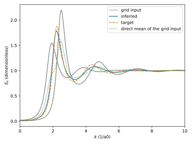
S_ii grid interpolation

More expensive calculation methods like DFT-MD or Average Atom can yield more accurate calculations for the static structure factors than the simpler models shipped with jaxrts. However, such simulations are normally only available on a grid. Hence, we provide a jaxrts.models.GridInterpolationSii class, interpolating with over such a grid. Centerpiece is the jaxrts.weissker_interpolator.SiiInterpolator, which implements the interpolation scheme proposed by [Weissker et al., 2009], lineraly interpolating the SSF’s integral over k, rather than the function ifself. However, as no sum rule exists for the SSFs, we interpolate the function’s norm, rather than putting it to a known value.

import jaxrts
from jaxrts.weissker_interpolator import AutoNormInterpolator
import jax.numpy as jnp
import matplotlib.pyplot as plt
from copy import deepcopy

ureg = jaxrts.ureg

state = jaxrts.PlasmaState(
    ions=[jaxrts.Element("Al")],
    Z_free=jnp.array([3]),
    mass_density=jnp.array([10]) * ureg.gram / ureg.centimeter**3,
    T_e=100 * ureg.electron_volt / ureg.k_B,
)
state["ion-ion Potential"] = jaxrts.hnc_potentials.YukawaShortRangeRepulsion(
    ureg("250pm")
)
state["ionic scattering"] = jaxrts.models.OnePotentialHNCIonFeat()

target_k, target_Sii = state["ionic scattering"].S_ii_on_grid(state)

# Create a 2x2 grid around the target state
T_range = 100 * ureg.electron_volt / ureg.k_B
rho_range = 8.0 * ureg.gram / ureg.centimeter**3

grid_Sii = jnp.zeros([*target_Sii.shape, 2, 2])
for idx in ([0, 0], [0, 1], [1, 0], [1, 1]):
    t, r = idx
    new_state = deepcopy(state)
    new_state.T_e += (t - 0.5) * T_range
    new_state.T_i = jaxrts.units.to_array([new_state.T_e])
    new_state.mass_density += (r - 0.5) * rho_range
    _, calc_Sii = new_state["ionic scattering"].S_ii_on_grid(new_state)
    grid_Sii = grid_Sii.at[:, :, :, *idx].set(
        calc_Sii.m_as(ureg.dimensionless)
    )

# Cut the grid at k == 10/a0
cutoff = 10 / ureg.a0
grid_Sii = grid_Sii[:, :, target_k < cutoff, :, :]
target_Sii = target_Sii[:, :, target_k < cutoff]
target_k = target_k[target_k < cutoff]


interpolator = AutoNormInterpolator(
    grid_Sii * ureg.dimensionless,
    target_k,
    state.T_e + (T_range * jnp.array([-0.5, 0.5])),
    state.mass_density[0] + (rho_range * jnp.array([-0.5, 0.5])),
)
# The second argument specifies the attributes of a plasma state that should be
# used when calling the `interpolator`.
# The syntax is either a plain attribute (`T_e`) or a jnpu function (`sum`) and
# then the :py:class:`jaxrts.plasmastate.PlasmaState` attributes that should be
# passed to that function (`mass_density`), separated by a '%'
Sii_model = jaxrts.models.GridInterpolationSii(
    interpolator, ["T_e", "sum%mass_density"]
)

k, Sii = Sii_model.S_ii_on_grid(state)
fig, ax = plt.subplots()
for idx in ([0, 1], [1, 0], [0, 0], [1, 1]):
    ax.plot(
        k.m_as(1 / ureg.a0),
        grid_Sii[0, 0, :, *idx],
        color="gray",
        label="grid input" if idx == [0, 0] else None,
        alpha=0.7,
    )
ax.plot(
    k.m_as(1 / (1 * ureg.a0)),
    Sii[0, 0, :].m_as(ureg.dimensionless),
    label="inferred",
)
ax.plot(
    k.m_as(1 / (1 * ureg.a0)),
    target_Sii[0, 0, :].m_as(ureg.dimensionless),
    ls="dashed",
    label="target",
)
ax.plot(
    k.m_as(1 / ureg.a0),
    (
        grid_Sii[0, 0, :, 0, 1]
        + grid_Sii[0, 0, :, 1, 0]
        + grid_Sii[0, 0, :, 0, 0]
        + grid_Sii[0, 0, :, 1, 1]
    )
    / 4,
    ls="dotted",
    label="direct mean of the grid input",
)
ax.set_xlabel("$k$ (1/a0)")
ax.set_ylabel("$S_{ii}$ (dimensionless)")
ax.set_xlim(0, 10)
plt.legend()
plt.tight_layout()
plt.show()