Comparison of different edge models

This example showcases different edge-models that can be used in the bound free scattering features.

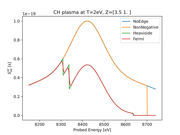
import matplotlib.pyplot as plt

# jax provides a submodule which can be (mostly) used as a drop-in replacement
# for numpy. We use jnp to avoid confusion.
from jax import numpy as jnp

import jaxrts

ureg = jaxrts.ureg

ions = [jaxrts.Element("C"), jaxrts.Element("H")]
rho = ureg("1g/cc")
number_fraction = jnp.array([1 / 2, 1 / 2])

Z_free = jnp.array([3.5, 1.0])
# ----------------------------------------------------------

measured_energy = jnp.linspace(5.5, 8.6, 4096) * ureg.kiloelectron_volt

mass_fraction = jaxrts.helpers.mass_from_number_fraction(number_fraction, ions)

state = jaxrts.PlasmaState(
    ions=ions,
    Z_free=Z_free,
    mass_density=rho * number_fraction,
    T_e=2 * ureg.electron_volt / ureg.k_B,
)

setup = jaxrts.Setup(
    scattering_angle=ureg("160deg"),
    energy=ureg("8700 eV"),
    measured_energy=ureg("8700 eV")
    + jnp.linspace(-550, 40, 500) * ureg.electron_volt,
    instrument=jaxrts.instrument_function.Gaussian(fwhm=ureg("5.0eV")),
)


for edge in [
    jaxrts.models.NoEdge,
    jaxrts.models.NonNegative,
    jaxrts.models.Heaviside,
    jaxrts.models.Fermi,
]:
    state["bf edge"] = edge()
    state["bound-free scattering"] = jaxrts.models.SchumacherImpulse()

    See_tot = state["bound-free scattering"].evaluate_raw(state, setup)

    plt.plot(
        setup.measured_energy.m_as(ureg.electron_volt),
        See_tot.m_as(ureg.second),
        label=edge.__name__,
    )
plt.xlabel("Probed Energy [eV]")
plt.ylabel("$S_{ee}^{bf}$ [s]")

plasma_str = "".join([i.symbol for i in state.ions])
plt.title(
    f"{plasma_str} plasma "
    + f"at T={(state.T_e * ureg.k_B).m_as(ureg.electron_volt):.0f}eV, "
    + f"Z={state.Z_free}"
)
plt.legend()
plt.show()